6. GEOG0027 (2020/1) Classification with Google Earth Engine (GEE)

This practical will use Google Earth Engine (GEE)’s python library EE and geemap library to automatically classify land covers and land uses in Shenzhen area. These two libraries are built to handle remote sensing (RS) data from the Cloud without physically downloading the data to our local computers, and they also allow easy python coding, where only small modifications are needed before handling large datasets. GEE hosts many popular RS datasets on the Cloud, and details of its data catalog can be found at: https://developers.google.com/earth-engine/datasets.

6.1. Jupyter setup

1. If you are using UCL’s Jupyter Hub (VPN or ChinaConnect required) to work with this chapter, please run the following command line in a Terminal first:*

conda config --add envs_dirs /shared/groups/jrole001/geog0027/envs/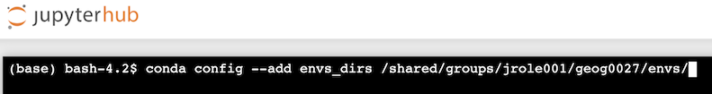

2. To download/clone the latest coursework notes, run the following command in a Terminal:

git clone -b 2020-2021 https://github.com/qwu-570/GEOG0027_Coursework.git

3. If you have cloned the git repository before, run the following command to update to the latest version:

git pull origin 2020-2021

4. Then, run source activate geemap in terminal to activate the geemap environment;

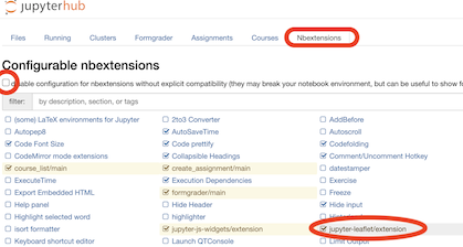
5. Run jupyter nbextension install --py --symlink --user ipyleaflet to install Leaflet extension, and then run jupyter nbextension enable ipyleaflet --user --py to enable the extension;

6. Close Terminal and double check if the jupyter-leaflet extension is enabled (especially if no visible output map from running the examples below):

6.2. First map

For the Shenzhen classification work, we start from displaying a basemap of the area. The first time when you use GEE, you will need to have a Google account and provide an authorization code as instructed.

import geemap, ee, os, numpy

Map = geemap.Map(center=[22.634, 114.19], zoom=9)
Map

A basic Google Map-like interface should be displayed here now. If you can’t see anything, please ensure that the ipyleaflet nbextension has been enabled.

6.3. Examining the time series

Let’s define a rectangular region of interest, following [min lon, min lat, max mon, max lat] first, and display a short ‘movie’ (a .gif file in fact) of how this area has changed over the past decades.

shenzhen_rec = ee.Geometry.Rectangle([113.7659, 22.40, 114.6654, 22.8536])

Map_gif = geemap.Map(center=[22.7511, 113.91], zoom=10)
Map_gif.add_landsat_ts_gif(roi=shenzhen_rec, start_year=1985, bands=['NIR', 'Red', 'Green'], frames_per_second=5)
Map_gif

Generating URL...
Downloading GIF image from https://earthengine.googleapis.com/v1alpha/projects/earthengine-legacy/videoThumbnails/110adcd928e58e193d881e403e07fd78-7e58ceab68ea08b9469270938f19c586:getPixels
Please wait ...
The GIF image has been saved to: /Users/qingling/Downloads/landsat_ts_yya.gif
Adding animated text to GIF ...
Adding GIF to the map ...
The timelapse has been added to the map.

The output map ‘Map_gif’ should look like something below.

Next, we will compare such change by using a slider

landsat_ts = geemap.landsat_timeseries(roi=shenzhen_rec, start_year=1986, end_year=2020, \
                                       start_date='01-01', end_date='12-31')

layer_names = ['Landsat ' + str(year) for year in range(1986, 2021)]

geemap_landsat_vis = {
    'min': 0,
    'max': 3000,
    'gamma': [1, 1, 1],
    'bands': ['NIR', 'Red', 'Green']} # You can change the vis bands here

Map2 = geemap.Map()
Map2.ts_inspector(left_ts=landsat_ts, right_ts=landsat_ts, left_names=layer_names, right_names=layer_names, \
                 left_vis=geemap_landsat_vis, right_vis=geemap_landsat_vis)
Map2.centerObject(shenzhen_rec, zoom=10)
Map2

We have previously defined a rectangle for Shenzhen area by coordinates, but we can also use existing shape/vector files to select Areas of Interest.

6.4. Select ‘Shenzhen’ as the area of interest (AOI)

The vector border layer is imported from https://developers.google.com/earth-engine/datasets/tags/borders, which includes the Global Administrative Unit Layers (GAUL) data from 2015. You may notice that Shenzhen’s boundary has expanded since (e.g. coastal landfill). We can, for example, manually draw/define another polygon and clip it to the GAUL border file, or, as a simple example, we will add a ‘buffer’ (e.g. 3000 meters) to the GAUL boundary data. This inevitably will introduce some areas outside the border of Shenzhen, e.g. part of Hong Kong, so you can work out some more elegant way of combining/clipping multiple AOI layers if time allows. Please justify your choice and summarize how you made it in the report. In the following example, I will use the shenzhen_buffer as my AOI.

cities = ee.FeatureCollection("FAO/GAUL/2015/level2")
#Map.addLayer(cities, {}, 'Cities', False)

shenzhen = cities.filter(ee.Filter.eq('ADM2_NAME', 'Shenzhen'))
outline = ee.Image().byte().paint(**{
  'featureCollection': shenzhen,
  'color': 1,
  'width': 3
})
Map.addLayer(outline, {}, 'Shenzhen')

# Next, add some buffer to include the coastal expansion areas
shenzhen_buffer = ee.Geometry(shenzhen.geometry()).buffer(3000)
Map.addLayer(shenzhen_buffer, {}, 'Buffer around Shenzhen')
#Map.addLayer(rec, "Original rec bounds")
#Map

6.5. Load Landsat data collections from GEE

Now we can see the the buffered AOI displayed on the Map. Next, let’s load some Landsat images for the Shenzhen area. I’ve defined here a python function called display_landsat_collection to do so. It automatically loads both the surface reflectance and annual NDVI image collections from GEE’s data catalog and also calculates the annual means for each band.

You can skip most of the details of what’s inside the code cell, but only to look at the first (and last) line of code. In order to run such function, you will need to choose a year (any year since 1984) and an AOI. In the following example, I choose year 2019 and the Shenzhen buffer to demonstrate the use of the code.

landsat_vis_param = {
            'min': 0,
            'max': 3000,
            'bands': ['NIR', 'Red', 'Green']  # False Colour Composit bands to be visualised
}
ndvi_colorized_vis = {
            'min': 0.0,
            'max': 1.0,
            'palette': [
            'FFFFFF', 'CE7E45', 'DF923D', 'F1B555', 'FCD163', '99B718', '74A901',
            '66A000', '529400', '3E8601', '207401', '056201', '004C00', '023B01',
            '012E01', '011D01', '011301']
}

def load_landsat_collection(year, aoi, cloud_tolerance = 3.0,
                            DISPLAY_ON_MAP = False, MEDIAN_ONLY = False):
    '''This function allows GEE to display a Landsat data collection
    from any year between 1984 and present year
    that fall within the AOI and cloud tolerance, e.g. 3.0%.
    There are two optional flag:
    When DISPLAY_ON_MAP is TRUE, display this layer onto Map;
    When return_series = 'MEDIAN_ONLY', only median SR is loaded into landsat_ts, and
    Setting this option to MEDIAN_ONLY would be faster than loading other collections.
    '''
    assert year >= 1984

    def renameBandsETM(image):
        if year >=2013: #LS8
            bands = ['B2', 'B3', 'B4', 'B5', 'B6', 'B7'] #, 'pixel_qa'
            new_bands = ['Blue', 'Green', 'Red', 'NIR', 'SWIR1', 'SWIR2'] #, 'pixel_qa'
        elif year <=1984:
            bands = ['B1', 'B2', 'B3', 'B4', 'B5', 'B7', 'pixel_qa']
            new_bands = ['Blue', 'Green', 'Red', 'NIR', 'SWIR1', 'SWIR2', 'pixel_qa']
        return image.select(bands).rename(new_bands)

    if not(MEDIAN_ONLY):
        if year >= 2013:
            layer_name = 'LC08' # LS8: 2013-now
        elif year == 2012: # # LS7: 1999- , however SLC error >= 1999:
            layer_name = 'LE07'
        elif year >=1984:
            layer_name = 'LT05' # LS5: 1984-2012

        collection_name_sr = f"LANDSAT/{layer_name}/C01/T1_SR"
        # You can also use the following line, if interested in incorperating ndvi
        collection_name_ndvi = f"LANDSAT/{layer_name}/C01/T1_ANNUAL_NDVI"

        all_sr_image = ee.ImageCollection(collection_name_sr) \
            .filterBounds(aoi) \
            .filterDate(f'{year}-01-01', f'{year}-12-31') \
            .filter(ee.Filter.lt('CLOUD_COVER', cloud_tolerance))\
            .sort('system:time_start') \
            .select('B[1-7]') \
            .sort('CLOUD_COVER')

        all_sr_image = all_sr_image.map(renameBandsETM) # rename bands with 'renameBandsETM' function

        # reduce all_sr_image to annual average per pixel
        mean_image = all_sr_image.mean()
        mean_image = mean_image.clip(aoi).unmask()

        ndvi_image = ee.ImageCollection(collection_name_ndvi)\
            .filterBounds(aoi) \
            .filterDate(f'{year}-01-01', f'{year}-12-31')\
            .select('NDVI')\
            .first()
        ndvi_image = ndvi_image.clip(aoi).unmask()

        #mean_image.addBands(ndvi_image, 'NDVI')

    # This line loads all annual median surface ref
    landsat_ts = geemap.landsat_timeseries(roi=shenzhen_buffer, start_year=year, end_year=year, \
                                       start_date='01-01', end_date='12-31')

    median_image = landsat_ts.first().clip(aoi).unmask()

    if DISPLAY_ON_MAP == True:

        if not(MEDIAN_ONLY):
            Map.addLayer(ndvi_image, ndvi_colorized_vis, 'NDVI '+str(year),  opacity=0.9)
            Map.addLayer(mean_image, landsat_vis_param, "Mean Ref "+str(year))
        Map.addLayer(median_image, landsat_vis_param, "Median Ref "+str(year))

    if MEDIAN_ONLY:
        return median_image
    else:
        return all_sr_image, mean_image, median_image, ndvi_image

Now the load_landsat_collection function has been defined, and we will run/execute it by calling the function name with appropriate input parameters (or ’arguments). The output of such function will be returned to the variables on the LHS of the equal sign, i.e. all_image_2019, mean_2019, median_2019, and ndvi_2019 in this case.

Map = geemap.Map(center=[22.634, 114.19], zoom=10)

# All you need to modify here is the YEAR below:
all_image_2019, mean_2019, median_2019, ndvi_2019 = load_landsat_collection(2019,\
                                        shenzhen_buffer, cloud_tolerance = 3,\
                                        DISPLAY_ON_MAP = True)
Map

You should examine the functions under the toolbar and layer buttons on the top-right corner of the Map, e.g. use the inspector and plotting tools to check the data values, or use layers control to switch on/off layers or to adjust opacity.

We can also check the metadata from the Landsat image collection we just loaded from the Cloud. Have a look of the output. Any useful information?

first_image = all_image_2019.first()

props = geemap.image_props(first_image)
print( props.getInfo())
#print(first_image.get('IMAGE_DATE').getInfo())
#print(first_image.get('CLOUD_COVER').getInfo(), '%')

{'CLOUD_COVER': 0.21, 'CLOUD_COVER_LAND': 0.23, 'EARTH_SUN_DISTANCE': 0.989463, 'ESPA_VERSION': '2_23_0_1b', 'GEOMETRIC_RMSE_MODEL': 7.889, 'GEOMETRIC_RMSE_MODEL_X': 5.66, 'GEOMETRIC_RMSE_MODEL_Y': 5.495, 'IMAGE_DATE': '2019-11-14', 'IMAGE_QUALITY_OLI': 9, 'IMAGE_QUALITY_TIRS': 9, 'LANDSAT_ID': 'LC08_L1TP_122044_20191114_20191202_01_T1', 'LEVEL1_PRODUCTION_DATE': 1575301122000, 'NOMINAL_SCALE': 30, 'PIXEL_QA_VERSION': 'generate_pixel_qa_1.6.0', 'SATELLITE': 'LANDSAT_8', 'SENSING_TIME': '2019-11-14T02:52:28.2228010Z', 'SOLAR_AZIMUTH_ANGLE': 153.700989, 'SOLAR_ZENITH_ANGLE': 45.366386, 'SR_APP_VERSION': 'LaSRC_1.3.0', 'WRS_PATH': 122, 'WRS_ROW': 44, 'system:asset_size': '627.230926 MB', 'system:band_names': ['Blue', 'Green', 'Red', 'NIR', 'SWIR1', 'SWIR2'], 'system:id': 'LANDSAT/LC08/C01/T1_SR/LC08_122044_20191114', 'system:index': 'LC08_122044_20191114', 'system:time_end': '2019-11-14 02:52:28', 'system:time_start': '2019-11-14 02:52:28', 'system:version': 1576236040308713}

Next, examine the mean, median surface reflectance and/or NDVI layers we’ve visualized. Which one is better? Which band should we include into the classification?

We can also use the Shenzhen GEE app from the previous chapter to examine the time series:

%matplotlib inline
from IPython.display import IFrame
IFrame('https://plewis.users.earthengine.app/view/shenzhen','100%',490)

In addition to switching layers on and off, adjusting opacity, we can also use python code to some simple mathmatical operations, e.g. calculating the differences:

mean_ndvi = mean_2019.normalizedDifference(['NIR', 'Red'])
median_ndvi = median_2019.normalizedDifference(['NIR', 'Red'])
median_ndwi = median_2019.normalizedDifference(['Green','NIR'])

Map.addLayer(mean_ndvi.subtract(median_ndvi), {'min': -0.2,'max': 0.2}, 'Diff in NDVI')
Map.addLayer(median_ndwi, ndvi_colorized_vis, 'NDWI from Meadian LS')
Map

6.6. K-means unsupervised classification with GEE

Let’s start with the 2019 Median image as an example. In the following code cell, a function named unsupervised_classifier has been defined to classify an image by take five input parameters (or ‘arguments’). You can don’t have to worry about the detail of the code except the very first line, where information about the ‘arguments’ can be found.

def unsupervised_classifier(image, aoi, year, n_clusters=5, output_filename='', DISPLAY_ON_MAP = False):
    '''This function provides a simple K-means classifier,
    with a default no. of cluster of 5. User will need to specify
    an AOI and an image to be classified.
    Optional arguments:
    n_clusters defines the number of clusters in the K-means classifier;
    output_filename should be a quoted string, e.g. 'Shenzhen_Landsat_Kmeans_2019.tif';
    DISPLAY_ON_MAP can be switched on, so the cluster map will be added to Map.
    '''

    # Make the training dataset:
    training_points = image.sample(**{
        'region': aoi,
        'scale': 30,
        'numPixels': 5000,
        'seed': 0,
        'geometries': True  # Set this to False to ignore geometries
    })

    #Map.addLayer(training_points, {}, 'training points', False) # No need to visualise this layer

    # Instantiate the clusterer and train it.
    clusterer = ee.Clusterer.wekaKMeans(n_clusters).train(training_points)

    # Cluster the input using the trained clusterer.
    class_result = image.cluster(clusterer)

    # Reclassify the map to avoid zero, in case of masking. E.g. from [0, 1, 2, 3, 4] to [1, 2, 3, 4, 5]
    #class_result = class_result.remap(list(range(0, n_clusters)), list(range(1, n_clusters+1)))

    if DISPLAY_ON_MAP:
        # Display the clusters with random colors.
        Map.addLayer(class_result.randomVisualizer(), {}, 'Clusters '+str(year), opacity=1.0)

    if output_filename == '':
        print(f'{year} classification finished. No output exported.')
    else:
        #Export the result directly to your computer/Hub:
        geemap.ee_export_image(class_result, filename=output_filename, \
                            scale=900, region=aoi, file_per_band=False)
        # When scale is small, GEE won't allow downloading due to size limitation

    return class_result

The above cell only ‘defines’ a function but does NOT execute it, so we now need to actually run it by calling the function name with appropriate arguments:

class_result = unsupervised_classifier(mean_2019, shenzhen_buffer, 2019, n_clusters=5, DISPLAY_ON_MAP = True)
Map

2019 classification finished. No output exported.

When we executed the unsupervised_classifier function, a variable class_result was used to received the returned values from the function, and we will use this class_result variable in the following code to inspect our classification output.

6.7. Link unsupervised clusters into Land Use Land Cover (LULC) classes

You need to carefully compare the K-means results with the original images to decide which cluster belongs to what class. Then, you can name the classes and assign appropriate RGB colours accordingly. However, the classified clusters may differ between different years, so you will need to change and classification setting (i.e. n_clusterss) and the legend for some of the years. Also, bare in mind, there might be mis-classified pixels. How can you improve the results?

legend_keys = ['Urban', 'Vegetation', 'Bright Urban',  'Water', 'Shaded Vegetation']
legend_colors = ['#FFFFB3', '#8DD3C7', '#FFFFB0','#80B1D3', '#8DD3C0']

Map.addLayer(class_result, {'min': 0, 'max': 4, 'palette': legend_colors}, 'Labelled clusters')
Map.add_legend(legend_keys=legend_keys, legend_colors=legend_colors, position='bottomright')

The number of clusters to use depends on the image, and it may different between different years. For the 2019 example, we used 5 clusters and the results seem to include two ‘Urban’ and two ‘Vegetation’ clusters. In such situation, we may consider grouping multiple clusters together, by re-mapping the cluster numbers:

# Reclassify the map. You may want to avoid zero, in case of masking.
remapped_class_result = class_result.remap([0, 1, 2, 3, 4], [1, 2, 1, 3, 2])

legend_keys = ['Urban', 'Vegetation', 'Water']
legend_colors = ['#FFFFB3', '#8DD3C7','#80B1D3']

Map.addLayer(remapped_class_result, {'min': 1, 'max': 3, 'palette': legend_colors}, 'Remapped clusters')
Map.add_legend(legend_keys=legend_keys, legend_colors=legend_colors, position='bottomright')

However, sometimes you may find the reclustered results less satisfactory, so consider carefully before executing the re-mapping code.

After remapping the clusters, we have just three final classes now. Would this be the same as if we ran the unsupervised_classifier function with n_clusters = 3? Have a try.

6.8. Cluster areas

Next, we need to find out the size of each cluster, i.e. how many pixels belong to each class, and the total size of each class (hint: how big is each pixel?)

def calculate_class_size(class_result, year, legend_keys, PRINT_STATS=False):
    n_clusters = len(legend_keys)

    #landsat_stats = geemap.image_stats(class_result, scale=90)
    #print(landsat_stats.getInfo())

    if year in [2000, 2004]:
        print(f'Downscaling for year {year}')
        scale_factor= 3
    else: scale_factor= 1

    stats = {'Year': year}
    for i in range(n_clusters):
        remap = numpy.zeros(n_clusters)
        remap[i] = 1
        class_0 = class_result.remap(list(range(0, n_clusters)), list(remap))
        #print(list(remap))
        class_stats0 = geemap.image_stats(class_0, scale=30*scale_factor)
        #print(class_stats0.getInfo())

        sum_class0 = class_stats0.getInfo()['sum']
        sum_clean = int(sum_class0['remapped'])
        if PRINT_STATS:
            print(legend_keys[i], 'has', sum_clean, 'pixles.')
        stats[legend_keys[i]] = sum_clean * (scale_factor**2)

    return stats

legend_keys = ['Urban', 'Vegetation', 'Bright Urban',  'Water', 'Shaded Vegetation']
stats_2019 = calculate_class_size(class_result, 2019, legend_keys, PRINT_STATS=True)

Urban has 1006156 pixles.
Vegetation has 821889 pixles.
Bright Urban has 374495 pixles.
Water has 901949 pixles.
Shaded Vegetation has 654431 pixles.

These are the numbers we will need for the R modeling. We will also show you how to export these values automatically later. But for now, have another close examination of the classification results and the functions we used to generated them.

6.9. Repeat for multiple years

By now, you should be able to understand that the load_landsat_collection function allows us to just vary the ‘year’ variable (and leave AOI and Cloud Tolerance constant) to loop through a time series of data. Similarly, for the unsupervised_classifier function, we can vary the input ‘image’ variable (an output from the load_landsat_collection function) in order to classify multiple images. Below is a loop built for running K-means classification for Landsat time series for the Shenzhen area. Years between 1987 to 2016 are selected to match our socio-economic data. When this cell is running (you can spot a star key on the LHS of the cell), you can track the progress by looking at the output messages. Once the cell finished running, an integer number will be shown outside of the LHS of the cell, and you can examine the layers in the Map (if DISPLAY_ON_MAP flag was set to True)

cluster_pixels = []

# Only to demonstrate every 10 years, but you should run every year, ideally in groups
for year in range(1986, 2017, 10):

    median_image = load_landsat_collection(year, shenzhen_buffer, cloud_tolerance=3,\
                                          MEDIAN_ONLY = True)
    class_result = unsupervised_classifier(median_image, shenzhen_buffer, year,\
                    n_clusters=5, DISPLAY_ON_MAP = True) #output_filename=f'Shenzhen_Landsat_Kmeans_{year}.tif'

    legend_keys = ['Class 1', 'Class 2', 'Class 3',  'Class 4', 'Class 5'] #change the class names

    stats = calculate_class_size(class_result, year, legend_keys)
    cluster_pixels.append(numpy.fromiter(stats.values(), dtype=int))
    #if 'Urban' in stats: print(f'There are {int(stats["Urban"])} urban pixles in {str(year)}.')
    print(stats)

#Map

1986 classification finished. No output exported.
{'Year': 1986, 'Class 1': 1295840, 'Class 2': 1137617, 'Class 3': 397936, 'Class 4': 679908, 'Class 5': 247620}
1996 classification finished. No output exported.
{'Year': 1996, 'Class 1': 1252350, 'Class 2': 1064788, 'Class 3': 382639, 'Class 4': 551019, 'Class 5': 508124}
2006 classification finished. No output exported.
{'Year': 2006, 'Class 1': 934998, 'Class 2': 830316, 'Class 3': 362536, 'Class 4': 860025, 'Class 5': 771044}
2016 classification finished. No output exported.
{'Year': 2016, 'Class 1': 620490, 'Class 2': 740670, 'Class 3': 488368, 'Class 4': 792561, 'Class 5': 1116831}

After running the above loop of code to classify a time series, all cluster areas (i.e. pixel counts) have been recorded into the cluster_pixels variable, and cluster layers are mapped into the Map.

6.10. Export results to excel (.csv) files

Lastly, we will use the following code to export the sizes of each class/cluster into a csv file, and you will need this file for R modeling in the next part of the coursework.

header = 'Year, ' + ', '.join( legend_keys )
numpy.savetxt("Shenzhen_pixel_stats.csv", cluster_pixels, delimiter=",", header=header)

Congratulations (on finishing the classification part)!

So far, we have processed the entire time series of Landsat data without actually downloading any of them to our local PC (everything is done on the Cloud!), except the .CSV file. I hope you’ve enjoyed playing with GEE here. Now you should be able to open the CSV file in excel or R to continue with the modeling part of the coursework.